Chapter 2 Introduction to the R-spatial ecosystem
2.1 R’s spatial ecosystem(s)
R is a powerful language for geocomputation, allowing for:
- Exploratory data analysis (EDA)
- Data processing (e.g., adding new variables)
- Data transformation (e.g., changing CRS, reducing size via simplification/aggregation)
- Data visualization
- Web application development
- Software development (e.g., to share new methods)
There are many ways to handle geographic data in R, with several dozens of packages in the area. It includes:
- {sf}, {sp}, {terra}, {raster}, {stars} - spatial classes
- {dplyr}, {rmapshaper} - processing of attribute tables/geometries
- {rnaturalearth}, {osmdata} - spatial data download
- {rgrass}, {qgisprocess}, {link2GI} - connecting with GIS software
- {gstat}, {mlr3}, {CAST} - spatial data modeling
- {rasterVis}, {tmap}, {ggplot2} - static visualizations
- {leaflet}, {mapview}, {mapdeck} - interactive visualizations
- {spatstat}, {spdep}, {spatialreg}, {dismo}, {landscapemetrics}, {RStoolbox}, {rayshader}, {gdalcubes}, {sfnetworks} - different types of spatial data analysis
- many more…
Visit https://cran.r-project.org/view=Spatial to get an overview of different spatial tasks that can be solved using R.
We think it is helpful to start learning the R-spatial ecosystem by using its packages for spatial classes handling. They offer capabilities to read/write spatial data, but also have many tools to process and transform the data. The below figure shows the change in popularity of the main R packages for spatial data handling – in this workshop, we will focus on {sf} for working with spatial vector data and {terra} for working with spatial raster data.
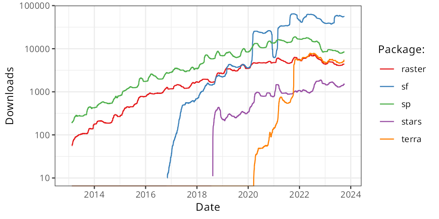
Figure 2.1: Source: https://geocompr.robinlovelace.net
2.2 Vector data
The {sf} package based on the OGC standard Simple Features. It allows to read, process, visualize, and write various spatial data files. As you can see in Figure 2.2, the {sf} package does not exist in void.

Figure 2.2: Source: https://www.r-spatial.org/r/2020/03/17/wkt.html
First, it is built upon several external libraries, including GDAL, PROJ, GEOS, and s2geometry. Second, it uses several R packages, such as {s2}, {units}, {DBI}. Third, it is a basis of a few hundred of other R packages.
{sf} represent all common vector geometry types (Figure 2.3): points, lines, polygons and their respective ‘multi’ versions. It also also supports geometry collections.
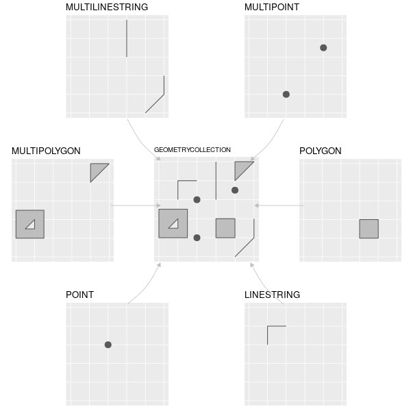
Figure 2.3: Source: https://geocompr.robinlovelace.net/spatial-class.html?q=sf%20classes#intro-sf
Most of the functions in this package start with a prefix st_:
## Linking to GEOS 3.10.2, GDAL 3.4.2, PROJ 7.2.0; sf_use_s2() is TRUE## [1] "%>%" "as_Spatial"
## [3] "dbDataType" "dbWriteTable"
## [5] "gdal_addo" "gdal_create"
## [7] "gdal_crs" "gdal_extract"
## [9] "gdal_inv_geotransform" "gdal_metadata"
## [11] "gdal_polygonize" "gdal_rasterize"
## [13] "gdal_read" "gdal_read_mdim"
## [15] "gdal_subdatasets" "gdal_utils"
## [17] "gdal_write" "gdal_write_mdim"
## [19] "get_key_pos" "NA_agr_"
## [21] "NA_bbox_" "NA_crs_"
## [23] "NA_m_range_" "NA_z_range_"
## [25] "pivot_wider.sf" "plot_sf"
## [27] "rawToHex" "read_sf"
## [29] "sf_add_proj_units" "sf_extSoftVersion"
## [31] "sf_proj_info" "sf_proj_network"
## [33] "sf_proj_pipelines" "sf_proj_search_paths"
## [35] "sf_project" "sf_use_s2"
## [37] "sf.colors" "st_agr"
## [39] "st_agr<-" "st_area"
## [41] "st_as_binary" "st_as_grob"
## [43] "st_as_s2" "st_as_sf"
## [45] "st_as_sfc" "st_as_text"
## [47] "st_axis_order" "st_bbox"
## [49] "st_bind_cols" "st_boundary"
## [51] "st_buffer" "st_cast"
## [53] "st_centroid" "st_collection_extract"
## [55] "st_combine" "st_contains"
## [57] "st_contains_properly" "st_convex_hull"
## [59] "st_coordinates" "st_covered_by"
## [61] "st_covers" "st_crop"
## [63] "st_crosses" "st_crs"
## [65] "st_crs<-" "st_delete"
## [67] "st_difference" "st_dimension"
## [69] "st_disjoint" "st_distance"
## [71] "st_drivers" "st_drop_geometry"
## [73] "st_equals" "st_equals_exact"
## [75] "st_filter" "st_geometry"
## [77] "st_geometry_type" "st_geometry<-"
## [79] "st_geometrycollection" "st_graticule"
## [81] "st_inscribed_circle" "st_interpolate_aw"
## [83] "st_intersection" "st_intersects"
## [85] "st_is" "st_is_empty"
## [87] "st_is_longlat" "st_is_simple"
## [89] "st_is_valid" "st_is_within_distance"
## [91] "st_jitter" "st_join"
## [93] "st_layers" "st_length"
## [95] "st_line_merge" "st_line_sample"
## [97] "st_linestring" "st_m_range"
## [99] "st_make_grid" "st_make_valid"
## [101] "st_minimum_rotated_rectangle" "st_multilinestring"
## [103] "st_multipoint" "st_multipolygon"
## [105] "st_nearest_feature" "st_nearest_points"
## [107] "st_node" "st_normalize"
## [109] "st_overlaps" "st_point"
## [111] "st_point_on_surface" "st_polygon"
## [113] "st_polygonize" "st_precision"
## [115] "st_precision<-" "st_read"
## [117] "st_read_db" "st_relate"
## [119] "st_reverse" "st_sample"
## [121] "st_segmentize" "st_set_agr"
## [123] "st_set_crs" "st_set_geometry"
## [125] "st_set_precision" "st_sf"
## [127] "st_sfc" "st_shift_longitude"
## [129] "st_simplify" "st_snap"
## [131] "st_sym_difference" "st_touches"
## [133] "st_transform" "st_triangulate"
## [135] "st_union" "st_viewport"
## [137] "st_voronoi" "st_within"
## [139] "st_wrap_dateline" "st_write"
## [141] "st_write_db" "st_z_range"
## [143] "st_zm" "vec_cast.sfc"
## [145] "vec_ptype2.sfc" "write_sf"Most often, the first step in spatial data analysis in R is to read the data. Here, we will read example file stored in the {spData} package:
## [1] "/Users/runner/work/_temp/Library/spData/shapes/world.gpkg"To read a spatial vector file, we just need to provide a file path to the read_sf() function:1
Our new object is an extended data frame with several non-spatial attributes and one special column geom.
When we print the object, it also provides a header with some basic spatial information:
## Simple feature collection with 177 features and 10 fields
## Geometry type: MULTIPOLYGON
## Dimension: XY
## Bounding box: xmin: -180 ymin: -89.9 xmax: 180 ymax: 83.64513
## Geodetic CRS: WGS 84
## # A tibble: 177 × 11
## iso_a2 name_l…¹ conti…² regio…³ subre…⁴ type area_…⁵ pop lifeExp gdpPe…⁶
## <chr> <chr> <chr> <chr> <chr> <chr> <dbl> <dbl> <dbl> <dbl>
## 1 FJ Fiji Oceania Oceania Melane… Sove… 1.93e4 8.86e5 70.0 8222.
## 2 TZ Tanzania Africa Africa Easter… Sove… 9.33e5 5.22e7 64.2 2402.
## 3 EH Western… Africa Africa Northe… Inde… 9.63e4 NA NA NA
## 4 CA Canada North … Americ… Northe… Sove… 1.00e7 3.55e7 82.0 43079.
## 5 US United … North … Americ… Northe… Coun… 9.51e6 3.19e8 78.8 51922.
## 6 KZ Kazakhs… Asia Asia Centra… Sove… 2.73e6 1.73e7 71.6 23587.
## 7 UZ Uzbekis… Asia Asia Centra… Sove… 4.61e5 3.08e7 71.0 5371.
## 8 PG Papua N… Oceania Oceania Melane… Sove… 4.65e5 7.76e6 65.2 3709.
## 9 ID Indones… Asia Asia South-… Sove… 1.82e6 2.55e8 68.9 10003.
## 10 AR Argenti… South … Americ… South … Sove… 2.78e6 4.30e7 76.3 18798.
## # … with 167 more rows, 1 more variable: geom <MULTIPOLYGON [°]>, and
## # abbreviated variable names ¹name_long, ²continent, ³region_un, ⁴subregion,
## # ⁵area_km2, ⁶gdpPercapIt is also possible to extract all of the spatial information with several specific functions.
For example, st_crs() is used to get information about the coordinate reference system of the given object:
## Coordinate Reference System:
##   User input: WGS 84
##   wkt:
## GEOGCRS["WGS 84",
##     DATUM["World Geodetic System 1984",
##         ELLIPSOID["WGS 84",6378137,298.257223563,
##             LENGTHUNIT["metre",1]]],
##     PRIMEM["Greenwich",0,
##         ANGLEUNIT["degree",0.0174532925199433]],
##     CS[ellipsoidal,2],
##         AXIS["geodetic latitude (Lat)",north,
##             ORDER[1],
##             ANGLEUNIT["degree",0.0174532925199433]],
##         AXIS["geodetic longitude (Lon)",east,
##             ORDER[2],
##             ANGLEUNIT["degree",0.0174532925199433]],
##     USAGE[
##         SCOPE["Horizontal component of 3D system."],
##         AREA["World."],
##         BBOX[-90,-180,90,180]],
##     ID["EPSG",4326]]
We can even extract different CRS definition with:
## [1] "GEOGCRS[\"WGS 84\",\n DATUM[\"World Geodetic System 1984\",\n ELLIPSOID[\"WGS 84\",6378137,298.257223563,\n LENGTHUNIT[\"metre\",1]]],\n PRIMEM[\"Greenwich\",0,\n ANGLEUNIT[\"degree\",0.0174532925199433]],\n CS[ellipsoidal,2],\n AXIS[\"geodetic latitude (Lat)\",north,\n ORDER[1],\n ANGLEUNIT[\"degree\",0.0174532925199433]],\n AXIS[\"geodetic longitude (Lon)\",east,\n ORDER[2],\n ANGLEUNIT[\"degree\",0.0174532925199433]],\n USAGE[\n SCOPE[\"Horizontal component of 3D system.\"],\n AREA[\"World.\"],\n BBOX[-90,-180,90,180]],\n ID[\"EPSG\",4326]]"## [1] "EPSG:4326"## [1] "+proj=longlat +datum=WGS84 +no_defs"We can quickly plot the object with the plot() function:
## Warning: plotting the first 9 out of 10 attributes; use max.plot = 10 to plot
## all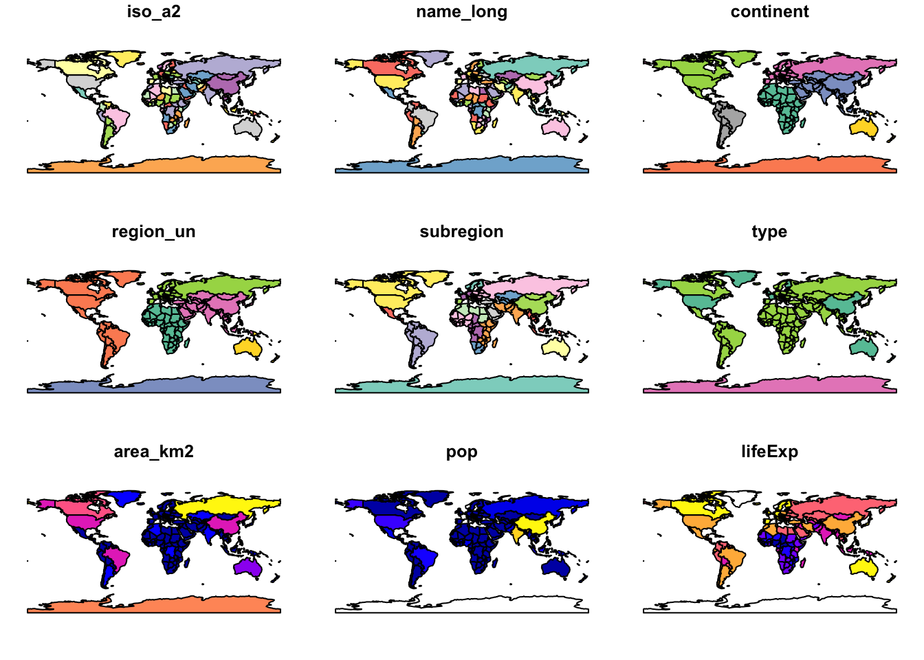
Let’s move to a different data example.
What to do when our data is stored in a text file (instead of a spatial file format)?
Then, we can read it as a regular data frame with read.csv:
cycle_hire_path = system.file("misc/cycle_hire_xy.csv", package = "spData")
cycle_hire_txt = read.csv(cycle_hire_path)
head(cycle_hire_txt)
## X Y id name area nbikes nempty
## 1 -0.10997053 51.52916 1 River Street Clerkenwell 4 14
## 2 -0.19757425 51.49961 2 Phillimore Gardens Kensington 2 34
## 3 -0.08460569 51.52128 3 Christopher Street Liverpool Street 0 32
## 4 -0.12097369 51.53006 4 St. Chad's Street King's Cross 4 19
## 5 -0.15687600 51.49313 5 Sedding Street Sloane Square 15 12
## 6 -0.14422888 51.51812 6 Broadcasting House Marylebone 0 18Next, we need to convert it into a spatial {sf} object with st_as_sf() by providing which columns contain coordinates, and what is the CRS of the data:
## Simple feature collection with 742 features and 5 fields
## Geometry type: POINT
## Dimension: XY
## Bounding box: xmin: -0.2367699 ymin: 51.45475 xmax: -0.002275 ymax: 51.54214
## Geodetic CRS: WGS 84
## First 10 features:
## id name area nbikes nempty
## 1 1 River Street Clerkenwell 4 14
## 2 2 Phillimore Gardens Kensington 2 34
## 3 3 Christopher Street Liverpool Street 0 32
## 4 4 St. Chad's Street King's Cross 4 19
## 5 5 Sedding Street Sloane Square 15 12
## 6 6 Broadcasting House Marylebone 0 18
## 7 7 Charlbert Street St. John's Wood 15 0
## 8 8 Lodge Road St. John's Wood 5 13
## 9 9 New Globe Walk Bankside 3 16
## 10 10 Park Street Bankside 1 17
## geometry
## 1 POINT (-0.1099705 51.52916)
## 2 POINT (-0.1975742 51.49961)
## 3 POINT (-0.08460569 51.52128)
## 4 POINT (-0.1209737 51.53006)
## 5 POINT (-0.156876 51.49313)
## 6 POINT (-0.1442289 51.51812)
## 7 POINT (-0.1680743 51.5343)
## 8 POINT (-0.1701345 51.52834)
## 9 POINT (-0.09644075 51.50739)
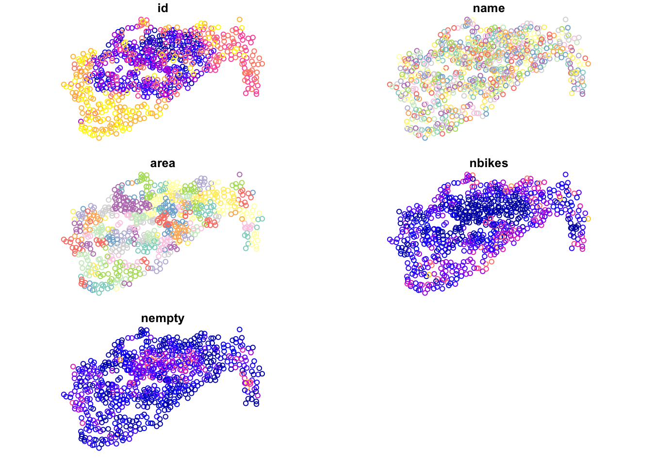
## 10 POINT (-0.09275416 51.50597)Now, we are able to plot and analyse the data:
We will give more example of the {sf} use in Chapter 4. To learn more read https://journal.r-project.org/archive/2018/RJ-2018-009/RJ-2018-009.pdf and visit https://r-spatial.github.io/sf/.
2.3 Raster data
The {terra} package contains classes and methods representing raster objects and operations. It allows raster data to be loaded and saved, provides raster algebra and raster processing, and includes a number of additional functions, e.g., for analysis of terrain characteristics. It also works well on large sets of data.
Similarly to {sf}, {terra} also uses many external libraries, but also enables many R packages (Figure 2.4).
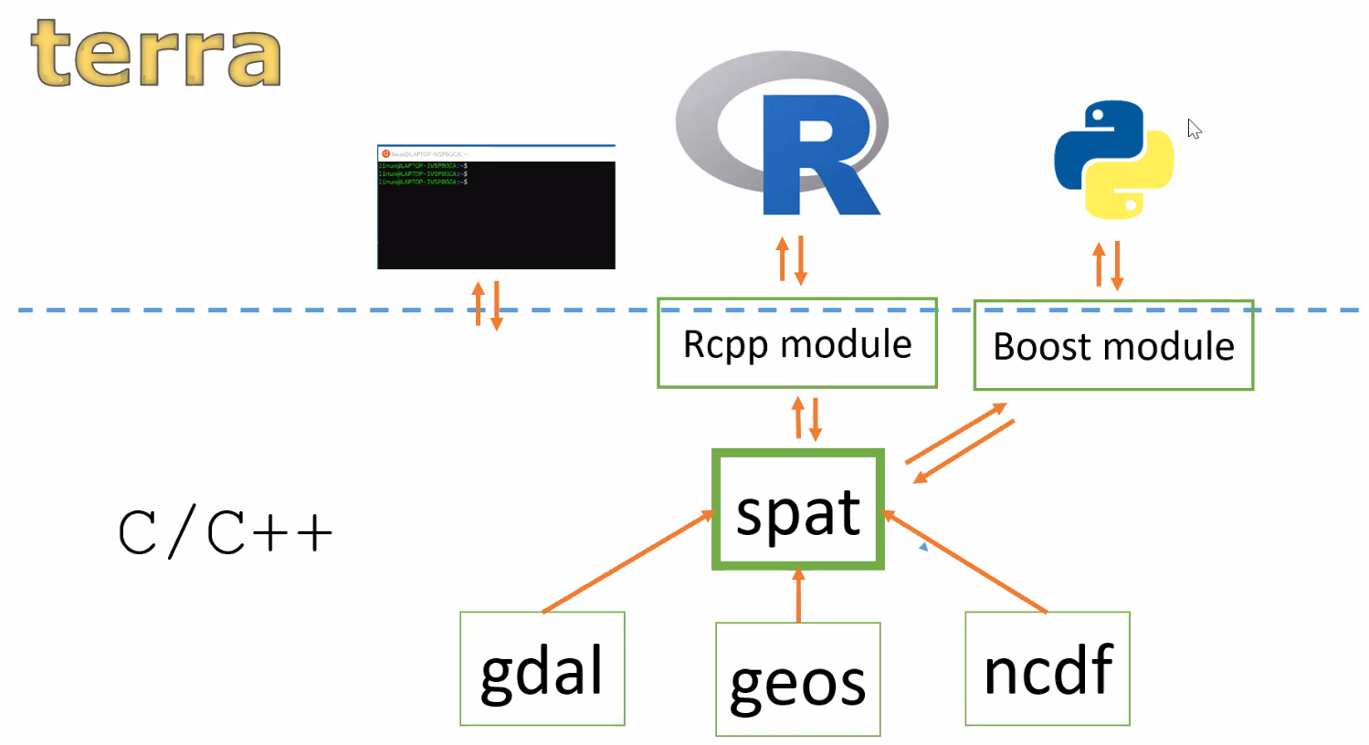
Figure 2.4: {terra} libraries
To read a spatial raster file, we just need to provide its file path to the rast() function:
## terra 1.6.11raster_filepath = system.file("raster/srtm.tif", package = "spDataLarge")
new_raster = rast(raster_filepath)Now, we can look at the summary of our data by typing the object’s name:
## class       : SpatRaster
## dimensions  : 457, 465, 1  (nrow, ncol, nlyr)
## resolution  : 0.0008333333, 0.0008333333  (x, y)
## extent      : -113.2396, -112.8521, 37.13208, 37.51292  (xmin, xmax, ymin, ymax)
## coord. ref. : lon/lat WGS 84 (EPSG:4326)
## source      : srtm.tif
## name        : srtm
## min value   : 1024
## max value   : 2892
It provides us information about the raster dimensions, resolution, CRS, etc.
crs() is used to get information about the coordinate reference system of the given {terra} object:
## [1] "GEOGCRS[\"WGS 84\",\n DATUM[\"World Geodetic System 1984\",\n ELLIPSOID[\"WGS 84\",6378137,298.257223563,\n LENGTHUNIT[\"metre\",1]]],\n PRIMEM[\"Greenwich\",0,\n ANGLEUNIT[\"degree\",0.0174532925199433]],\n CS[ellipsoidal,2],\n AXIS[\"geodetic latitude (Lat)\",north,\n ORDER[1],\n ANGLEUNIT[\"degree\",0.0174532925199433]],\n AXIS[\"geodetic longitude (Lon)\",east,\n ORDER[2],\n ANGLEUNIT[\"degree\",0.0174532925199433]],\n ID[\"EPSG\",4326]]"## name authority code area extent proj
## 1 WGS 84 EPSG 4326 <NA> NA, NA, NA, NA +proj=longlat +datum=WGS84 +no_defsWe are also able to create quick visualization with plot():
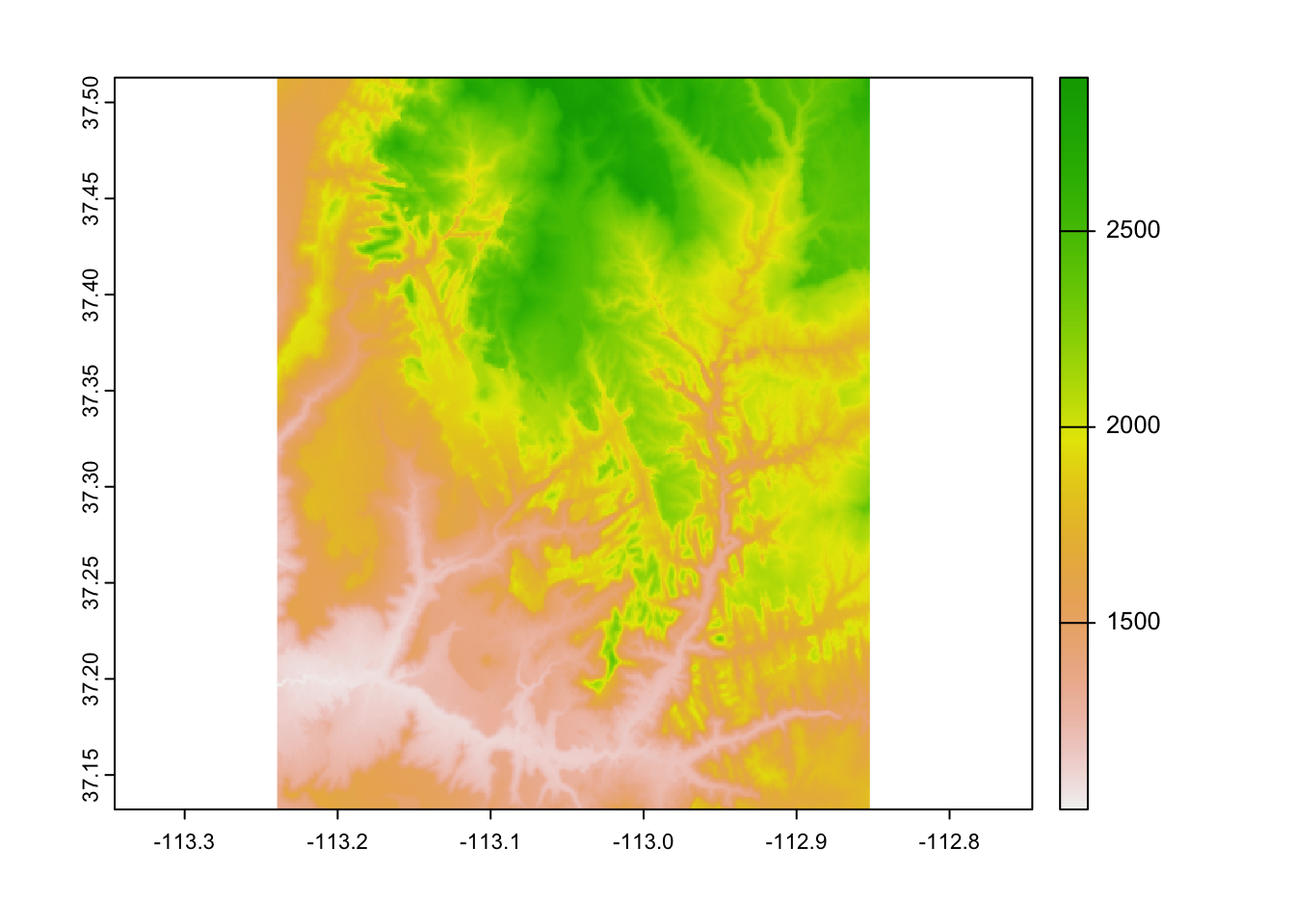
The {terra} package also supports multi-layered raster files.
For example, the landsat.tif file has four bands:
raster_filepath2 = system.file("raster/landsat.tif", package = "spDataLarge")
new_raster2 = rast(raster_filepath2)
plot(new_raster2)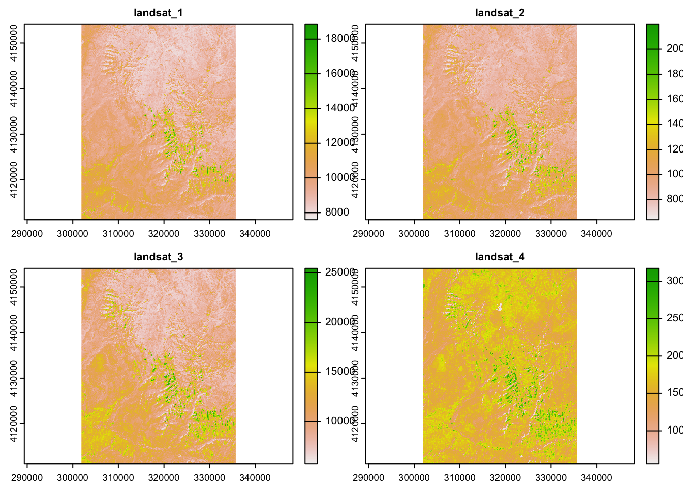
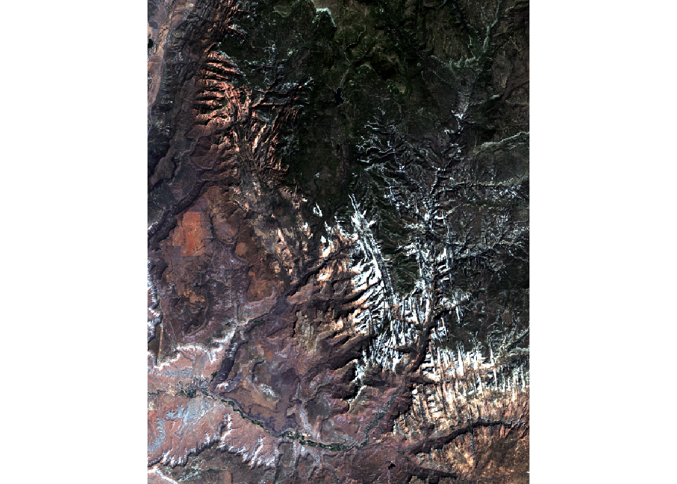
In this case, we are also able to plot three layers with plotRGB():
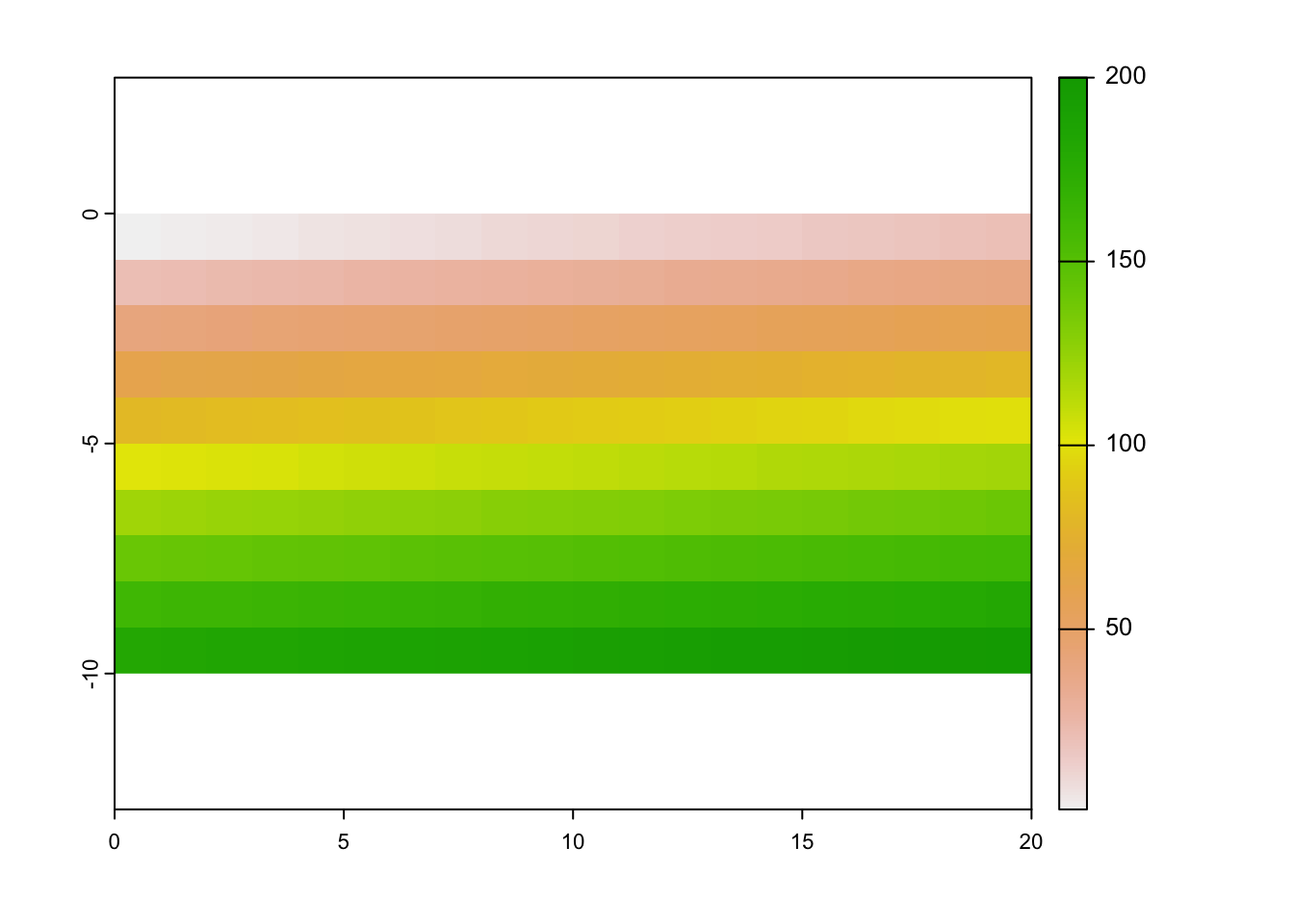
Sometimes, we want to create a raster from scratch.
This is also possible with the rast() function:
my_raster = rast(nrows = 10, ncols = 20, xmin = 0, xmax = 20, ymin = -10, ymax = 0,
                 crs = "EPSG:4326", vals = 1:200)
my_raster
## class : SpatRaster
## dimensions : 10, 20, 1 (nrow, ncol, nlyr)
## resolution : 1, 1 (x, y)
## extent : 0, 20, -10, 0 (xmin, xmax, ymin, ymax)
## coord. ref. : lon/lat WGS 84 (EPSG:4326)
## source : memory
## name : lyr.1
## min value : 1
## max value : 200Let’s plot our new object:
We will give more example of the {terra} use in Chapter 5.
To learn more about the package type ?terra or visit https://rspatial.github.io/terra/reference/terra-package.html.
There is also a second similar function allowing to read spatial vector files called
st_read().↩︎